As part of our blog series on Regional Risk Index and Epidemiology modelling, here are two blogs on the Effective Reproduction Number.
The Effective Reproduction number is covered in two blogs:
- The first blog described the calculation methodology for Germany (see: Calculation of the effective reproduction number – Germany)
- This second blog will cover the generalization of the previous methodology globally and the reproduction number forecasting.
Objective
As already described in the first blog, we need to look at the same metrics as governments do, in order to be able to understand and later foresee government decisions on lockdown measures, Among others as active case numbers or intensive care units, this is also the (effective) reproduction number. This can then also be used as an input for the epidemiological model and provides a more realistic value compared to a model-based assumption.
Data Sources
For the global calculation one needs to combine multiple data sources to be able to calculate the effective reproduction number. For each country one needs the overall case numbers and a so-called patients line list. In these line lists there is one row per person, with one column for the reporting date and one column for the symptom’s onset date. This information originates from questionnaires, which patients were asked to answer when being tested for COVID19. For various reasons this data is not only quite rare, but also it is extremely country specific and not easy to find. Also combining these data for multiple countries into one source is a non-trivial task. One research group (Open COVID-19 Data Working Group), who invested a lot of work and effort published a global line list on github [1] [2] with the data catalogue published here [3]. This data source for a global patients line list in combination with the global case numbers provided by Johns Hopkins University [4] is the base for the calculation of the effective reproduction number. The calculation procedure is performed in accordance with the procedure published by Robert Koch Institute, described in this article [5] as well as in this article [6] and also in other sources, for example here [7].
Generalizing globally
Where possible, so where a representative amount of the overall case numbers has given a symptoms onset date, the country specific delay distribution is calculated. For example, this is possible for Germany or Japan with more than 60% of the cases with a given symptoms onset case. Unfortunately, there are a lot of countries, for which only few cases have a given symptoms onset date (For instance Italy has 244216 confirmed cases (as of 2020-07-20) but only 3 rows for patients in the global line list with given symptoms onset and reporting date). For these countries a global delay distribution is used. This one is based on all cases world-wide, for which a symptoms onset is given, or rather for which the symptoms onset date is given in the source provided by the Open COVID-19 Data Working Group. Altogether these are 261335 cases (as of 2020-07-20). This global delay distribution can be seen here:
![A chart showing the global delay histogram and fitted Weibull distribution calculated from all cases with given reporting and symptoms onset date in the global patients line list provided by the Open COVID-19 Data Working Group [1]](https://emergentalliance.org/wp-content/uploads/2021/01/Global_Delay_Distribution.png)
The global delay histogram and fitted Weibull distribution calculated from all cases with given reporting and symptoms onset date in the global patients line list provided by the Open COVID-19 Data Working Group [1]
Calculation Procedure
The user of the notebook can select the country of interest, for which the calculation should be performed with a box-select widget.
Apart from the aligning of the data sources, thus mapping of the country names, the calculation procedure consists of four steps:
1. Construct a line list and fit the delay distribution
For each country the overall number of cases and the number of cases with given symptoms onset date are read. If for less than 10% of the cases a symptoms onset date is given, the global delay distribution is used.
For the confirmed cases a line list is constructed from the overall case numbers and the reporting date given in the data from Johns Hopkins University. For each day as many rows as number of new cases are appended with the respective reporting date and missing symptoms onset. Then for all available entries in the global line list for this specific country the respective symptoms onset date is pasted into the country specific line list. So, for the datapoints for which both dates are given the delay distribution can then be fitted. As described in [7, 2, 6] a Weibull distribution is supposed to give a good fit.
2. Imputation
This delay distribution is then applied to the datapoints with missing symptoms onset date. A reporting delay according to the delay distribution is assigned to these datapoints and from there the respective symptoms onset date is calculated.
3. Nowcasting
The same distribution is then used to adapt the case numbers to account for the cases which according to the delay distribution will be reported in the future with symptoms onset date until today. The python routine, which was used for the nowcasting, originates here [8].
4. Calculation of the effective reproduction number with a rolling window ratio
The calculation of the effective reproduction number itself is performed as a summation of case numbers for a specific amount of days and subsequently calculating the ratio between two sums. The proper selection of this series of intervals requires epidemiological domain knowledge and is fundamental for the sensitivity of the calculated data.
We ran the calculations with 7 days intervals, according to this publication by Robert Koch Institute [6].
Validation of the results
For the countries, which do publish their effective reproduction number a validation can be performed. This was done for Germany. The resulting numbers were in very good agreement with the officially published numbers. It could be shown that the quality of the resulting numbers is depending on the amount of data provided. For validation we also calculated the effective reproduction number for Germany with the global delay distribution, assuming we would not have enough data for a country specific delay distribution, and this resulted in a very poor agreement with the official numbers.

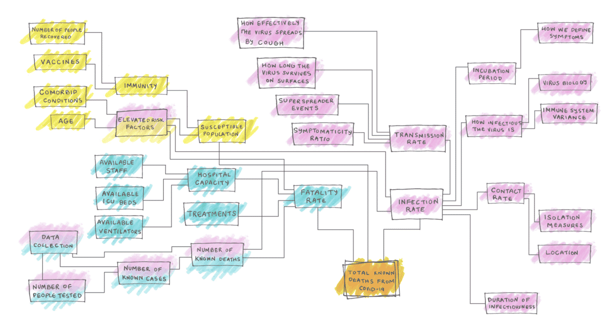
Picture from [9, 10]
Among lots of other factors one can imagine that especially the counter measures introduced by the governments and the mobility have a huge impact onto the growth rate, ergo the reproduction number. Also, not only the status quo and the current government measures, which are in place, are important, but also the evolution of the pandemic and the history of events. With the discussed model we aim to take into account the historic time series data and predict the effective reproduction number for the next days.
Data Sources
We use three different data sources for feature generation:
- Global case numbers published by John Hopkins University [4]
- Google mobility report, which quantifies the relative change in mobility behaviour [10]
- Stringency Index published by University of Oxford, which quantifies the government measures [10, 8, 4, 3, 5]
Calculation Procedure
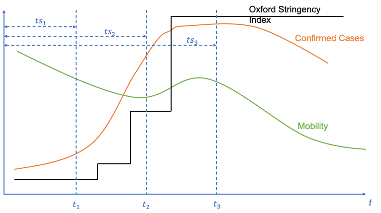
For feature generation we use the tsfresh package [12] , to extract time series features like e.g. mean value or absolute sum of changes. We perform this time series feature extraction for all three data sources. To account for the evolution of the time series, we use all datapoints up to the selected point in time. So, for day n we use all datapoints in the time series starting with day 0 until day n. Day 0 is defined as the “outbreak” point in time, when the first 100 confirmed cases were reported for the respective country. This approach also means that the time series for feature generation for day n+1 inherits the time series taken for day n. For the label of day n we use the effective reproduction number calculated for day n+x with x being the number of days which we aim to forecast. x should also be a meaningful value representing the duration between causing variables and the measurable impact onto the reproduction number. By this we achieve the forecasting functionality and account for the time delay between cause and effect. An illustration of the described approach can be seen here:
The effective reproduction number can be calculated with the help of imputation and nowcasting up to today. But for detecting possible clusters and regions with local outbreaks we need to be able to forecast the reproduction number. The modelling of this number is really hard, as it depends on various inputs, as described for example in this article [9] showing the complexity and the huge amount of impacting factors.

Time series taken into account for tsfresh feature generation for every day since the first 100 confirmed cases were reported for the country
Features, extracted for all time series (Confirmed Cases, Mobility, Oxford Stringency Index)
X (Confirmed Cases, …)=f1(ts1) f1(ts2) f1(ts3) f2(ts1) f2(ts2) f2(ts3) f3(ts1) f3(ts2) f3(ts3)
Labels
y=reff (t1) reff (t2) reff (t3)
After a feature selection, a linear regression model is trained on the dataset for day 0 until today minus 30 days and tested for the last 30 days until today.
Validation
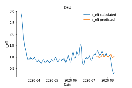
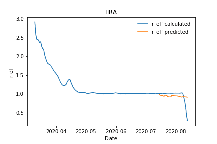
The predictions for Germany and France are in good agreement, whereas for example the predictions for UK differ from the real values. One major reason for this deviation has its root cause in the quality of the data, which was used for the label calculation itself. As explained in detail in the previous section, the available data differs extremely between the countries, resulting in different confidence for the labels, the calculated effective reproduction numbers, which we calculated in this notebook upfront for the respective country.

Calculated vs predicted effective reproduction number for Germany

Calculated vs predicted effective reproduction number for France
The code for the described calculation can be found in our GitHub repository.
We are a team of data scientists from IBM’s Data Science & AI Elite Team, IBM’s Cloud Pak Acceleration Team, and Rolls-Royce’s R2 Data Labs working on Regional Risk-Pulse Index: forecasting and simulation within Emergent Alliance. Have a look at our challenge statement!
Author
Astrid Walle is an AI Dev Specialist at R2 Data Labs at Rolls Royce Deutschland Ltd
The work was done in collaboration with Kyuhwa Lee and Sarah Boufelja, who are members of the IBM Data Science & AI Elite Team, as well with Klaus Paul, head of Berlin AI Hub at R2 Data Labs .
Special thanks to Erika Agostinelli and Mehrnoosh Vahdat.
Disclaimer: This information can be used for educational and research use. Please note that this analysis is made on a subset of available data. The authors do not recommend generalising the results and conclude decision-making on these sources only.
Works Cited
| 1 | Open COVID-19 Data Working Group, “Detailed Epidemiological Data from the COVID-19 Outbreak,” 2020. [Online]. Available: http://virological.org/t/epidemiological-data-from-the-ncov-2019-outbreak-early-descriptions-from-publicly-available-data/337. [Accessed 08 2020]. |
| 2 | Open COVID-19 Data Working Group, “Detailed Epidemiological Data from the COVID-19 Outbreak,” 2020. [Online]. Available: https://github.com/beoutbreakprepared/nCoV2019. [Accessed 08 2020]. |
| 3 | B. Xu, B. Gutierrez, S. Mekaru, K. Sewalk, L. Goodwin, A. Loskill, E. Cohn, Y. Hswen, S. C. Hill, M. M. Cobo, A. Zarebski, S. Li, C.-H. Wu and E. Hulland, “Epidemiological data from the COVID-19 outbreak, real-time case information,” Scientific Data, vol. 07, 2020. |
| 4 | COVID-19 Data Repository by the Center University, “JHU CSSE COVID-19 Data,” [Online]. Available: https://github.com/CSSEGISandData/COVID-19. |
| 5 | M. an der Heiden and O. Hamouda, “Schätzung der aktuellen Entwicklung der SARS-CoV-2- Epidemie in Deutschland – Nowcasting,” Epidemiologisches Bulletin, vol. 17, pp. 10-15, 2020. |
| 6 | Robert-Koch-Institut, Erläuterung der Schätzung der zeitlich variierenden Reproduktionszahl R, 2020. |
| 7 | S. Gloeckner, G. Krause and M. Hoehle, “Now-casting the COVID-19 epidemic: The use case of Japan, March 2020,” medRxiv, vol. 03, no. 18, 2020. |
| 8 | K. Systrom, T. Vladek and M. Krieger, “rt.live,” Github repository, no. https://github.com/rtcovidlive/covid-model, 2020. |
| 9 | M. Koerth, L. Bronner and J. Mithani, “Why It’s So Freaking Hard To Make A Good COVID-19 Model,” 31 03 2020. [Online]. Available: https://fivethirtyeight.com/features/why-its-so-freaking-hard-to-make-a-good-covid-19-model/. |
| 10 | University of Oxford, “CORONAVIRUS GOVERNMENT RESPONSE TRACKER,” [Online]. Available: https://www.bsg.ox.ac.uk/research/research-projects/coronavirus-government-response-tracker. [Accessed 08 2020]. |
| 11 | Google, “See how your community is moving around differently due to COVID-19,” 2020. [Online]. Available: https://www.google.com/covid19/mobility/. [Accessed 08 2020]. |
| 12 | M. Christ and e. al., “tsfresh,” [Online]. Available: https://tsfresh.readthedocs.io/en/latest/text/introduction.html. [Accessed 08 2020]. |

