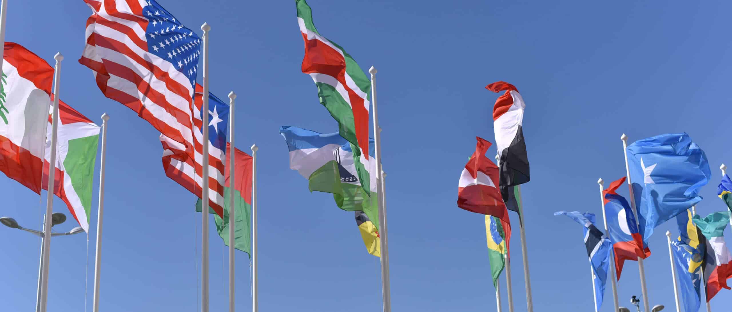
The COVID-19 crisis is affecting the globe in terms of public health, governmental restrictions and interventions, effects on personal freedom and opinion, mobility, and, last but not the least, economy. Trying to understand the interactions between these aspects is extremely complex. For the purpose of modelling the health status, but also to be able to make use of data such as mobility, we decided to build a geospatial knowledge graph to understand countries and their relationships.
Encountering Geo Data
We normally work with time series, IoT style data from machines and equipment. Some of our equipment is used to transport passengers where we encounter location information, but, in those circumstances, geo data are relatively well-defined (airports or train stops).
When embarking on this project we began to realise that global geospatial data can be challenging. Early on, we started to create initial mapping tables to be able to display the excellent Johns Hopkins Center for Systems Science and Engineering (CSSE) data onto choropleth maps of the world – both datasets had different names for the same country in many cases, as it turned out.
As we continued our journey in analysing more and more datasets we encountered an ever growing list of names and standards. There are ISO 3 Character, ISO 2 Character codes, ISO numeric, FIPS, NUTS, numerical codes, hierarchical codes, and many, many ways in spelling one country’s name.
After many iterations we finally settled for the following main sources for geospatial data:
- pycountry, a well maintained python package
- naturalearth.com, for geographic data
- various national data sources for individual countries
There exist many other, very useful data sources such as gadm, United Nations, World Bank, some of which were used to manually assemble the country cross reference table on Github.
Geographical Context from Geo Data
Our project aims to model and understand the effects of the COVID-19 pandemic. One workstream specifically focusses on local risk indices. For this use case, we need the notion of borders, and regions that share a border. It is important to have a concept of what we call a cell. This is a geographical entity, such as a country, a nation, a federation or a republic. As it turned out, this is not well defined.
Soon, this caused another challenge, that of the abstract level of countries, departments, states, regions, districts or countries. It was fairly obvious when we worked with the first data sources, that, as an example, the United Kingdom comprises England, Scotland, Wales, and Northern Ireland. What came as a surprise was the variety of what these entries are called.
For the EU, a scheme called NUTS (Nomenclature of territorial units for statistics) is available. This follows a logic of abstraction levels, and, in our project, we tried to use that nomenclature as much as we could.
That did not consider another aspect that was new to us: overseas territories. The most prominent example in the context of the COVID-19 pandemic was that, when analysing digital data, France was bordering Brasil, and Suriname, by virtue of French Guiana. There are many more examples similar to this, such as Spain and Morocco via Ceuta, UK and Spain via Gibraltar, to name a few. Luckily, the border between St. Marteen and St. Martins did not create a new border relationship.
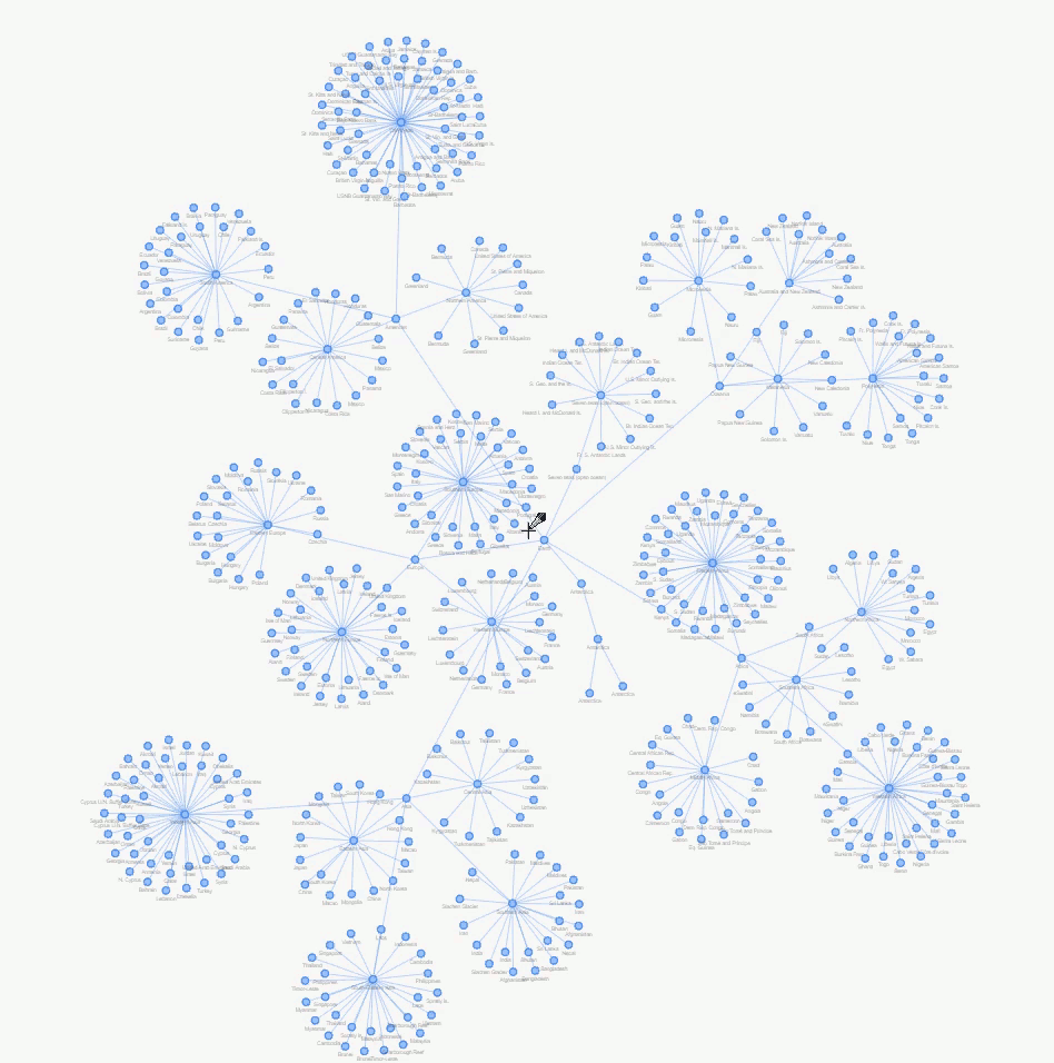
As our context clearly has to do with actual geographical neighbourhood, we settled for using the nartualearth Sovereignity dataset. This gave a good starting point for creating a knowledge graph of the “as intended” world, as the data are logically structured by entities and sub-entitites, such as continents, sub-regions, and countries.To build a knowledge graph, we use python NetworkX package, which offers data structures and tools to create nodes and edges, i.e. connections between nodes. All of these can have attributes, such as names. In the case of the edges, we followed the schema.org standard for countries and labelled parent-child relationships as “containsPlace”, i.e. “Western Europe containsPlace Germany”. This produces a beautiful network graph when visualising it with the python pyvis package, which allows for interaction with the plot.
Computing Neighbourhood Relationships
The world knowledge graph does not yet contain an actual representation of which countries actually share borders. Using geopandas as the data source, and geojson and shapefiles as data sources, this can readily be computed by checking if the map vector data of two countries, or regions, share commonality. This article was our initial inspiration.
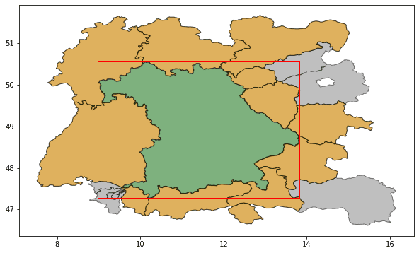
It is very inefficient to compute neighbourhood relations at a global level as most countries, or regions, will have a relatively low number of neighbour cells. Fortunately, geopandas allows specifying a bounding box on its read_file method, this significantly reduces computational time as only a shortlist of candidates need to be loaded.So, as an example, if we want to compute all neighbours of Bavaria at the same level of abstraction (let’s call this abstraction region ignoring that Bavaria is a state), we can compute the bounding box of Bavaria first.
gf = gpd.read_file("naturalearthdata.com_downloads/ne_10m_admin_1_states_provinces.shp")
gfBavaria = gf[gf.iso_3166_2 == "DE-BY"]
x0,y0,x1,y1 = gfBavaria.geometry.bounds.values[0]
gfNeighbours = gpd.read_file("naturalearthdata.com_downloads/ne_10m_admin_1_states_provinces.shp", bbox=(x0,y0,x1,y1))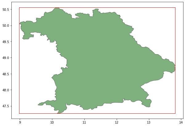
Fig. 2 Bavaria and its geospatial bounding box shown as a red rectangle
This already drastically reduced the load time and memory footprint of the geodata to be used in the next step. The candidate neighbours are given in the table below. Also note that Bavaria/Bayern is shown again, as it, obviously is in its own bounding box.
| ISO 3166-1 alpha-2 | Region Name |
| CH | Appenzell Ausserrhoden |
| CH | Appenzell Innerrhoden |
| DE | Baden-Württemberg |
| DE | Bayern |
| DE | Hessen |
| CZ | Jihočeský |
| CZ | Karlovarský |
| AT | Oberösterreich |
| CZ | Plzeňský |
| DE | Sachsen |
| AT | Salzburg |
| CH | Sankt Gallen |
| AT | Steiermark |
| CZ | Středočeský |
| CH | Thurgau |
| DE | Thüringen |
| AT | Tirol |
| AT | Vorarlberg |
| CS | Ústecký |
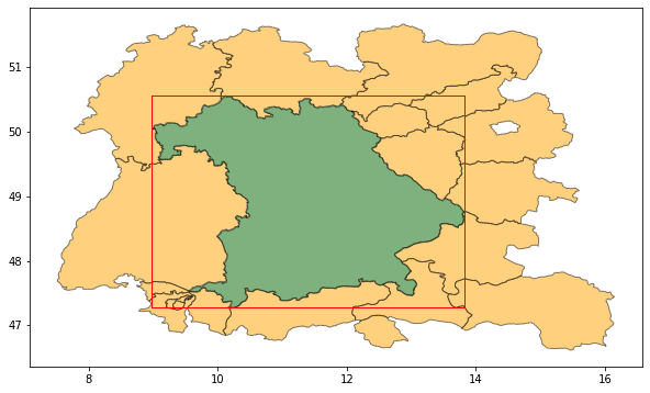
Fig. 3 Bavaria, its bounding box, and the regions loaded by geopandas after applying the bbox filter
The final step now computes if, for each region, the border vector data touches the border vector data of Bavaria. This removes regions such as the Swiss regions in the SW, which are in the bounding box initially, and regions that are behind immediate neighbours, and produces the correct result once Bavaria has been removed from the result set.
| ISO 3166-1 alpha-2 | Region Name |
| DE | Baden-Württemberg |
| DE | Hessen |
| CZ | Jihočeský |
| CZ | Karlovarský |
| AT | Oberösterreich |
| CZ | Plzeňský |
| DE | Sachsen |
| AT | Salzburg |
| DE | Thüringen |
| AT | Tirol |
| AT | Vorarlberg |
Bavaria and its direct neighbours it shares a land border with
The above can also be represented as a neighbourhood graph which will also show the neighbourhood relationships between the neighbouring regions.

Fig. 5 Graph network of Bavaria and its neighbours and their respective neighbouring relation
Performing this computations for all Admin 1 level entries of the naturalearth dataset results in 21800 neighbourhood relationships at that level. Unfortunately, we could only perform spot checks on the data. The results do not appear to be 100% accurate in that they lack some neighbourhood relationships in South Korea, but they would not introduce non-existent neighbourhoods as was the case, unfortunately, with the gadm dataset, where we found pointers to inconsistencies and workarounds late in the project.
Putting it together
During computation of the neighbourhood relations we now also compute the length of the border, and the compass orientation of the neighbourhood relationship. This is being computed by computing the centroid of the border polygon. Data are created as compass orientation, North being 0, E 90, and S being 180.
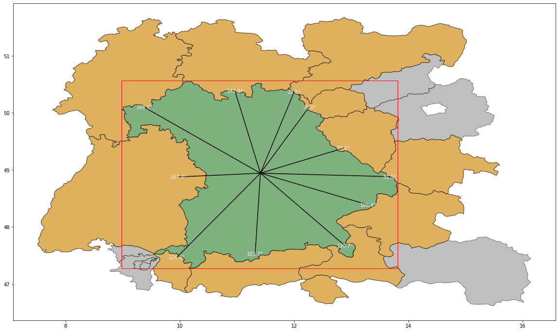
Fig. 6 Bavaria and its neighbouring states including their compass directions
Knowing the “direction” of neighbours around a region will allow meaningful ways of visualising possible. One example which we will try to investigate if the infection numbers are transported across boundaries, and how much a border between an entity influences the infection propagation. As one example, the heatmap below show, for Potsdam SE of Berlin, the currently used metric of number of new cases summed over the last seven days. Potsdam is at the top of the heatmap, its neighbours are arranged clockwise beginning with its southern neighbour, the Potsdam-Mittelmark region.
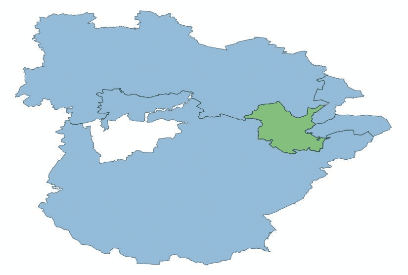
Fig. 7 Postdam (green) surrounded by (clockwise from 1 o’clock) Berlin Spandau, Berlin Steglitz-Zehlendorf, LK Potsdam-Mittelmark, and LK Havelland
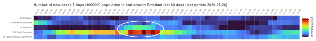
Fig. 8 An attempt to semantically arrange neighbouring regions. Potsdam is in the centre of a “new cases reported last 7 days” heatmap, surrounded by its neighbours. The marked area (white circle) shows a possible co-occurence of infection numbers between Berlin Spandau and Havelland, with Falkensee and Spandau being very close neighbours.
Conclusion
We all use services such as Google Maps or Apple Maps or SatNav systems in cars and take their map data for granted. Diving into geospatial data proved to be a journey in data engineering, schemas, standards, and levels of abstractions. On my (data) journeys, I have come across very remote islands, some uninhabited, territories under dispute and countries last encountered in history classes at school.
For us, handling graph data and knowledge graphs will become a major part of our work at R² Data Labs. Gaining experience in this, and also a better understanding on how to perform data management and the use of standards such as those from schema.org will help us in our everyday business.
Last but not least, adding the notion of neighbours adds a novel viewpoint to analyses done around the COVID-19 crisis. Most statistics are done at national (or country, see the discussion above) level, but closure of borders may become necessary as the world tries to contain the spread of the virus.
Disclaimer: This information can be used for educational and research use. Please note that this analysis is made on a subset of available data. The author does not recommend generalising the results and conclude decision-making on these sources only.
Author
Dr. Klaus G. Paul is Head of Berlin AI Hub and Emerging Technologies Capabilities Lead at R² Data Labs, Rolls-Royce Deutschland
Many thanks to my collaborators from the IBM Elite team on this project, and their ideas and feedback, as well as my immediate colleagues from the R²Data Labs Berlin, Bangalore, and London AI Hubs.